Part 1
- 試寫一函數 regPolygon(n),其功能為畫出一個圓心在 (0, 0)、半徑為 1 的圓,並在圓內畫出一個內接正 n 邊形,其中一頂點位於 (1, 0)。例如 regPolygon(8) 可以畫出如下之正八邊型:
- 一條參數式的曲線可由下列方程式表示:
x = sin(t), y = 1 - cos(t) + t/10 當 t 由 0 變化到 4*pi 時,請寫一個 MATLAB 的腳本 plotParam.m,畫出此曲線在 XY 平面的軌跡。
- 試寫一函數 regStar(n),其功能為畫出一個圓心在 (0, 0)、半徑為 1 的圓,並在圓內畫出一個內接正 n 星形,其中一頂點位於 (1, 0)。例如 regStar(7) 可以畫出如下之正 7 星型:
- 一個平面上的橢圓可以表示成下列方程式:
(x/a)2+(y/b)2=1 我們也可以用參數式將橢圓表示成:x = a*cos(t) 請利用上述參數式,寫一個函數 ellipse(a, b),其功能是畫出一個橢圓,而且橢圓上共有100個點。例如,ellipse(7, 2) 可以產生下列圖形:
y = a*sin(t)
- 請用寫一個 MATLAB 腳本 figSolve.m,利用圖解法,說明下列聯立方程式有無窮多組解:
y = x (請務必畫出上述兩條曲線來加以說明之。)
y = sin(1/x)
- 利薩如圖形(Lissajous Figure,又稱為 Bowditch Curve)可用下列參數式來表示:
x = cos(m*t) 試畫出在不同 m、n 值的利薩如圖形:
y = sin(n*t)- m = n = 1
- m = 3, n = 2
- m = 2, n = 7
- m = 10, n = 11
- Chebyshev 多項式的定義如下:
y = cos(m*cos-1x) 其中 x 的值介於 [-1, 1]。當 m 的值由 1 變化到 5,我們可得到五條曲線。請將這五條曲線畫在同一張圖上面,記得要使用 legend 指令來標明每一條曲線。
- 使用 MATLAB 畫一個圓心在原點、半徑等於 10 的圓,並在圓周上依逆時鐘方向取 任意四點 A、B、C、D,將線段 AB、AC、AD、BC、BD、CD 用直線畫出。
- 計算線段 AB、AC、AD、BC、BD、CD 的長度。
- 計算 AB*CD+AD*BC 和 AC*BD。兩者的差距有多少?是否可視為相等?
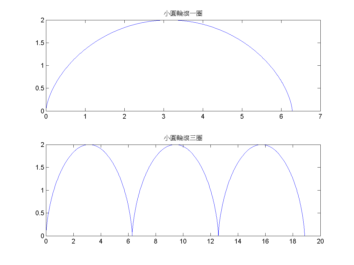
- 當一個小圓輪在平面上滾動時,輪緣的一點在滾動時所形成的軌跡稱為「擺線」(Cycloid)。請用 MATLAB 畫出一個典型的擺線,其中小圓輪的半徑為 1,而且至少要滾三圈。產生圖形如下:
- 此題和上題類似。當一個小圓輪沿著一條曲線行進時,輪緣任一點的軌跡就會產生變化豐富的擺線。假設小圓輪的半徑 r=2。
- 當小圓輪繞著一個大圓(半徑 R=5)的外部滾動時,請畫此「圓輪擺線」或「外花瓣線」。
- 重複上小題,但改成在大圓的內部滾動,請畫出此「內花瓣線」。
- 若大圓和小圓的半徑成整數比,當小圓在大圓的內部滾動時,小圓內的任一點 A 的軌跡就會形成一個漂亮無缺的花瓣線。當大圓半徑 R 為 10,小圓半徑 r 為 3,且 A 點離小圓圓心距離 r1 為 2 時,請畫出此完整的花瓣線。
Part 2
- Simple plots by hands:
Please presume you are MATLAB to plot the result of the following commands using a pen. Here we have a = [1 2; 3 4].
(Please remember to write down the coordinates of the endpoints of each line.)
- plot(a);
- plot(a');
- plot(a, a');
- plot(a, a', a', a);
- Ellipse plots by hands:
Please presume you are MATLAB to plot the result of the following commands using a pen. Here we have t = linspace(0, 2*pi).
- x=cos(t); y=sin(t); plot(x, y);
- x=cos(t); y=2*sin(t); plot(x, y);
- x=2*cos(t); y=sin(t); plot(x, y);
- Lissajous figures by hands:
Please presume you are MATLAB to plot the result of the following commands using a pen. Here we have t = linspace(0, 2*pi).
- x=cos(t); y=sin(t); plot(x, y);
- x=cos(t); y=sin(2*t); plot(x, y);
- x=cos(2*t); y=sin(t); plot(x, y);
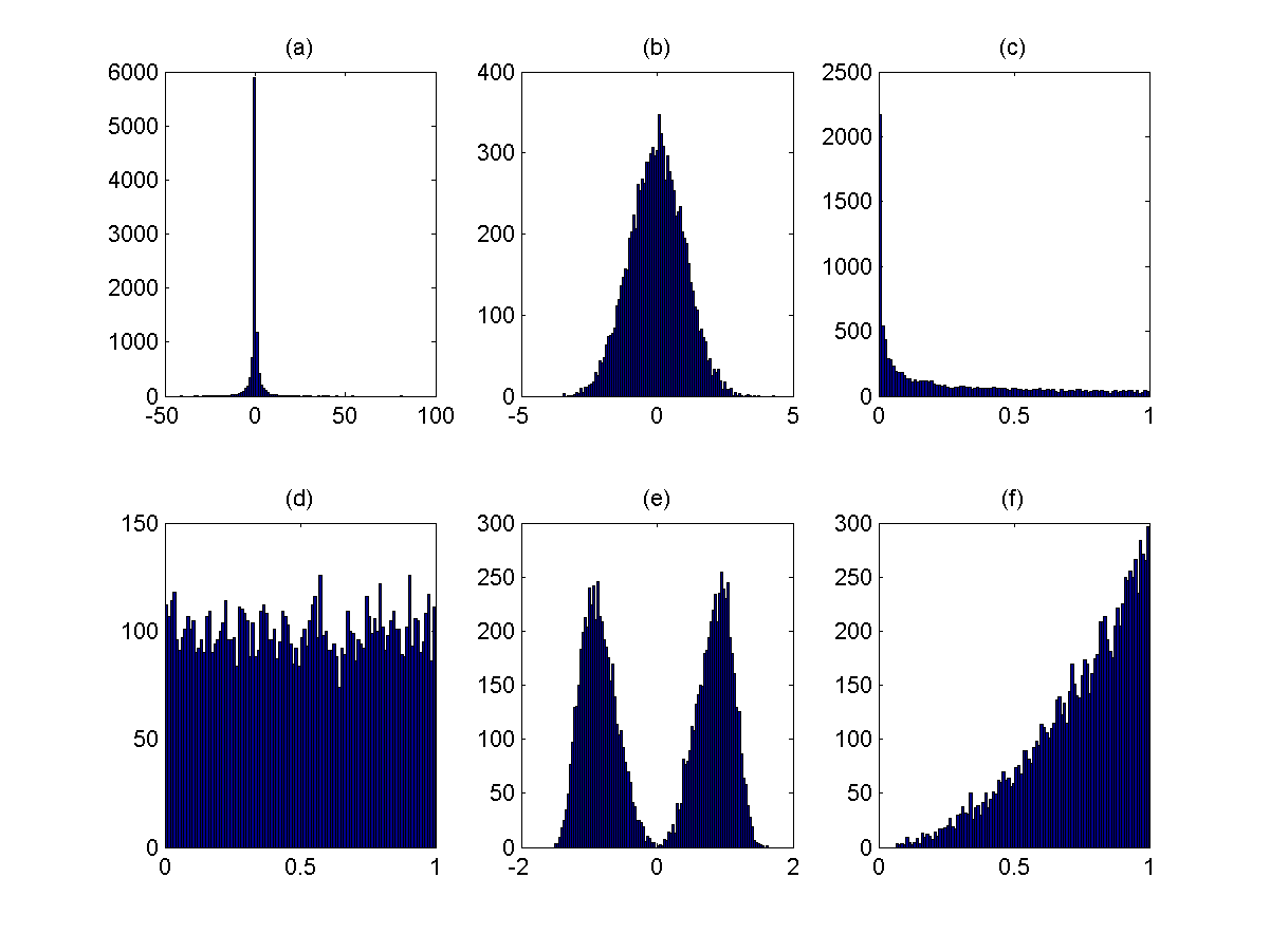
- Histogram plots:
Determine which one of the following plot is most likely to be generated by each of the following commands:
- x=rand(10000, 1); hist(x, 100);
- x=randn(10000, 1); hist(x, 100);
- x=rand(10000, 1); hist(x.^3, 100);
- x=randn(10000, 1); hist(x.^3, 100);
- x=rand(10000, 1); hist(nthroot(x, 3), 100);
- x=randn(10000, 1); hist(nthroot(x, 3), 100);
- Euler's formula:
- What is Euler's formula?
- How can you prove it? (Hint: Use Taylor series expansion.)
- Use the formula to prove that $e^{i\pi}+1=0$.
- Use the formula to prove that $\cos(3\theta)=4 \cos(3\theta)-3 \cos \theta$.
- Equivalence between polar and plot:
Explain why the following two commands will generate same plot (on different coordinate systems), assuming θ is a vector and r(θ) is a function of θ.
- polar(θ, r(θ));
- plot(r(θ).*exp(j*θ));
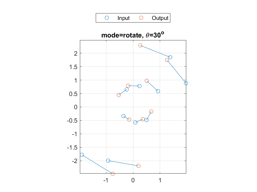
- Rotation and reflection:
Write a MATLAB function myTransform.m to rotate or reflect a set of 2D points. The usage of the function is
output=myTransform(vec, theta, mode) where- vec: a 2-by-n vector representing n points in 2D space
- theta: angle (counter-clockwise, in radian) for rotation or reflection. For rotation, theta is the rotation angle. For reflection, it is the angle of the reflection axis.
- mode: 'rotate' for rotation, 'reflect' for reflection
- output: a 2-by-n vector representing the given n points after rotation or reflection
Here is a test case for 'rotate':
- Inputs:
- vec=[-0.235892197136722 1.96453251156114 0.0845369570761526 0.499750630743405 0.238445635648528 0.924272931895896 1.3779342772046 -1.89766476744468 -0.922641236606734 -0.357100057722689;0.652821094952841 0.884584173475766 -0.574514061258489 -0.484104482611851 0.778248191474934 0.588137914293571 1.85120493279698 -1.77868417910781 -1.99792708362756 -0.336400759888822];
- theta=pi/6;
- mode='rotate';
- Output:
- output=[-0.530699182751349 1.25904297483451 0.360468183015827 0.674848983087011 -0.182624117844313 0.506374881905385 0.267723622406047 -0.754083806919876 0.19993279233326 -0.141057341736327;0.447413553787173 1.74833862179625 -0.455275293343144 -0.169371464656083 0.793205522090853 0.971478840654975 2.29215763801555 -2.48921806813918 -2.19157622763379 -0.469881632777453].
And here is a test case for 'reflect':
- Inputs:
- vec=[-1.39813787581107 0.164404073318729 -0.273046949402907 -0.480937151778845 0.664734120627595 0.880952785381048 -0.784146183664088 1.85859294855571 0.103359722310648 0.113596996734002;-0.255055179880806 0.747734028808123 1.57630014654608 0.327512120829686 0.0851885927211602 0.323213137847597 -1.80537335138609 -0.604530088774459 0.563166955145978 -0.904726212798032];
- theta=pi/3;
- mode='reflect';
- Output:
- output=[0.478184672761947 0.565354627562556 1.50163944559949 0.524102392575249 -0.258591574904627 -0.160565604477623 -1.17142609378376 -1.4528348885086 0.436037028573025 -0.840314382119783;-1.338350508386 0.51624511838372 0.551684478664278 -0.252747730649369 0.618270931586387 0.924534060598447 -1.58177719102676 1.30732366435664 0.371095622822115 -0.353985221433752].
(Note that the plots are only for reference. You don't need to generate the plots.)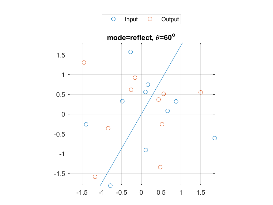
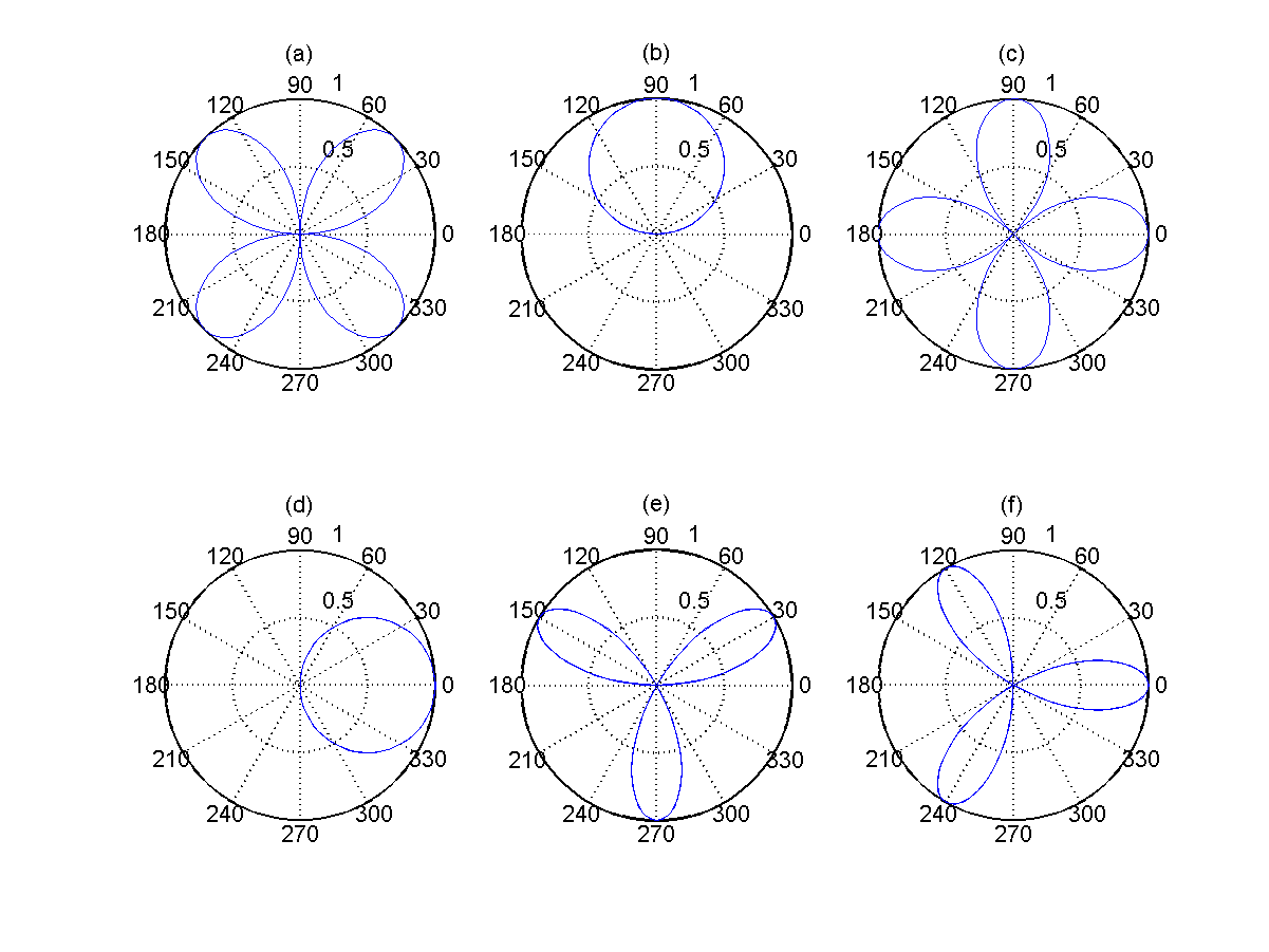
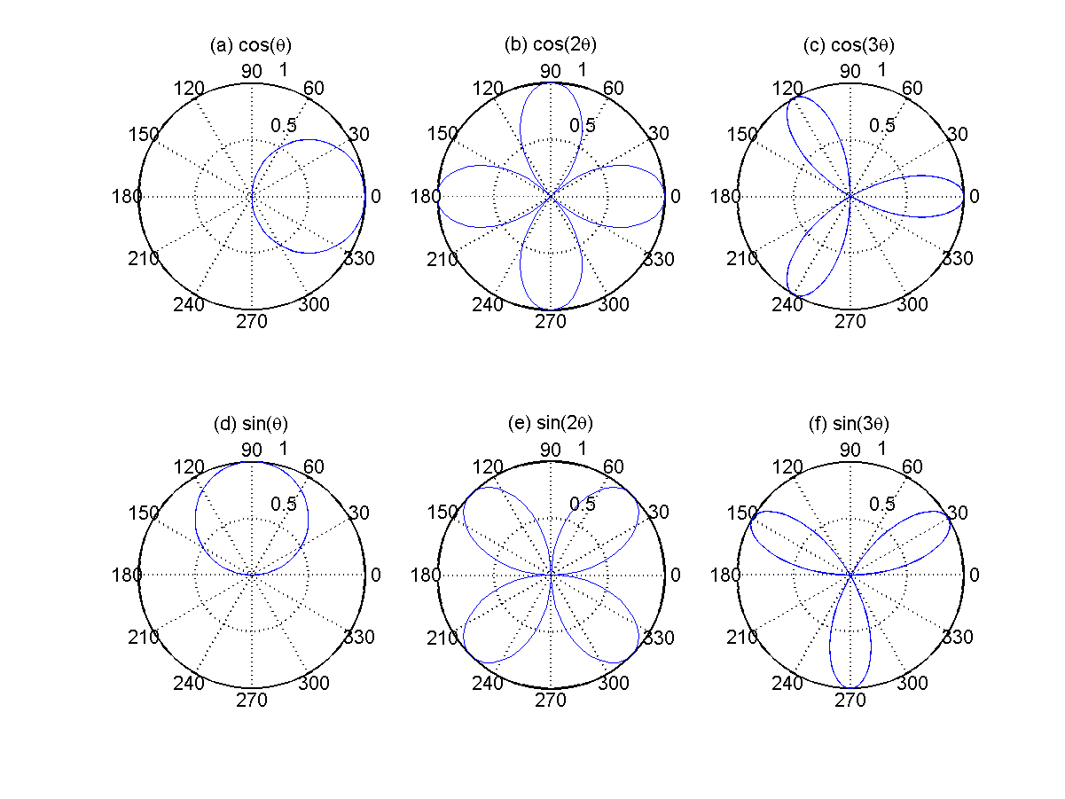
- Plots of rose curves:
Determine which one of the following plot is most likely to be generated by each of the following commands:
- theta=linspace(0, 2*pi); polar(theta, cos(theta));
- theta=linspace(0, 2*pi); polar(theta, sin(theta));
- theta=linspace(0, 2*pi); polar(theta, cos(2*theta));
- theta=linspace(0, 2*pi); polar(theta, sin(2*theta));
- theta=linspace(0, 2*pi); polar(theta, cos(3*theta));
- theta=linspace(0, 2*pi); polar(theta, sin(3*theta));
- Sketch of rose curves:
Please use the method of "描點作圖" to sketch the following rose curves in the polar coordinate system, assuming the range of θ is between 0 and 2*pi.
- r = cos(θ)
- r = cos(2θ)
- r = cos(3θ)
- r = sin(θ)
- r = sin(2θ)
- r = sin(3θ)
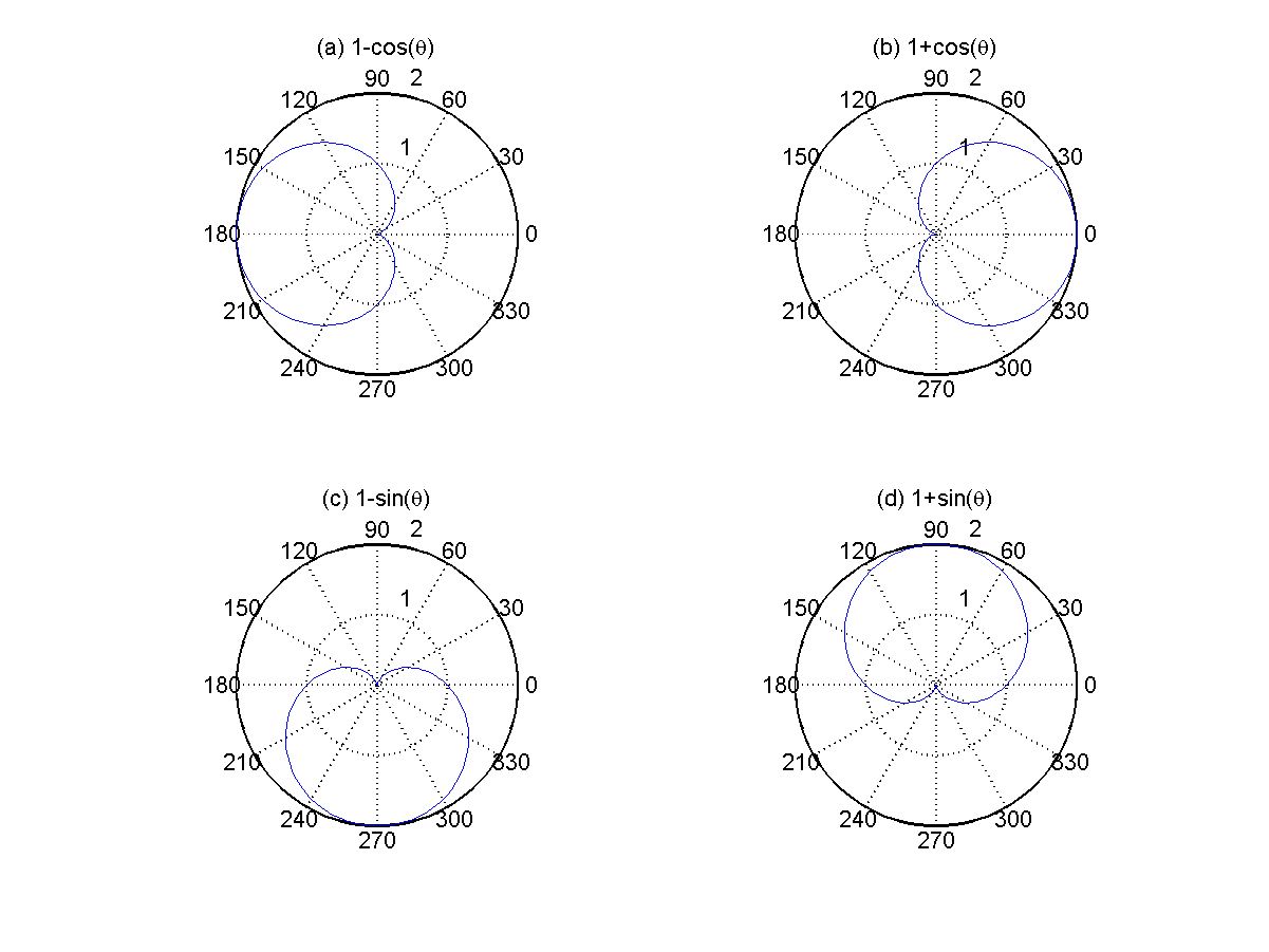
- Sketch of cardioids:
Please use the method of "描點作圖" to sketch the following cardioids (心臟線) in the polar coordinate system, assuming the range of θ is between 0 and 2*pi.
- r = 1 - cos(θ)
- r = 1 + cos(θ)
- r = 1 - sin(θ)
- r = 1 + sin(θ)
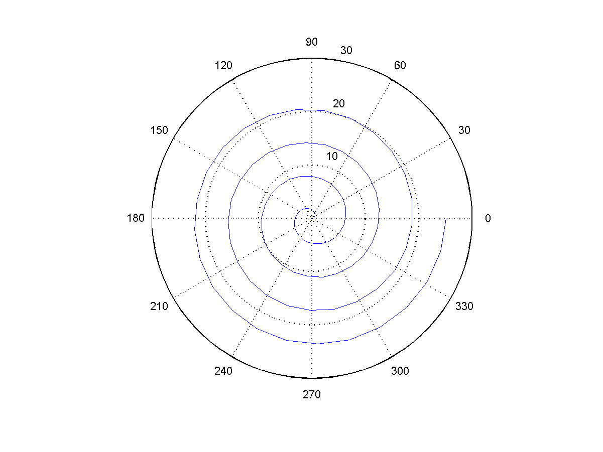
- Plot of a simple spiral:
請使用 MATLAB 的兩個指令,分別在平面上畫出螺旋圖,從原點開始,逐漸向外繞圈擴散,圖形如下。(提示:若以極座標來想像,則 r 和 θ 都是必須是隨時間而遞增的函數。)
- 使用 plot 指令,畫出圖形如下:
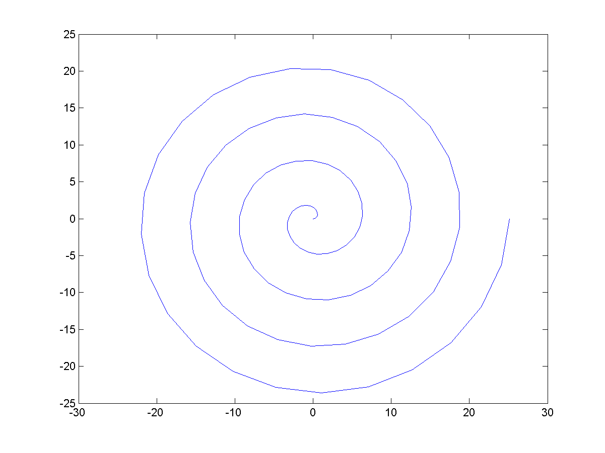
- 使用 polar 指令,畫出圖形如下:
- 使用 plot 指令,畫出圖形如下:
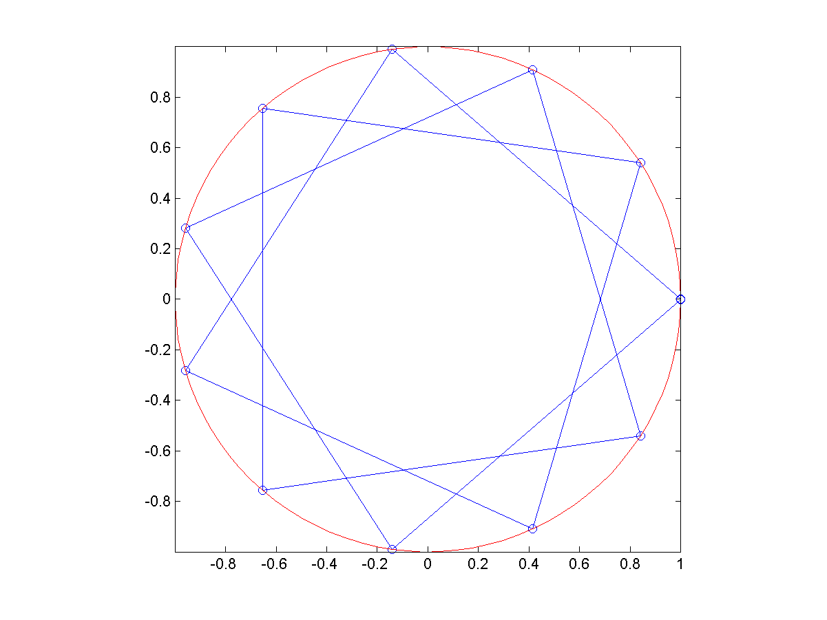
- Plot general regular stars:
- 試寫一函數 regGeneralStar(n, k),其功能為畫出一個圓心在 (0, 0)、半徑為 1 的圓,並在圓內畫出一個內接星形,其中一頂點位於 1+0*i(複數表示法),下一頂點則位於 exp(i*2*pi*k/n),依此類推。例如 regGeneralStar(11, 3) 可以畫出如下之圖形:
- Please try the following code to show some animation:
for i=1:1000
	regGeneralStar(79, i);
	drawnow
end
Please convert the animation into an animated gif file, using any resources you can find over the internet. You gif file should look like this:
- 試寫一函數 regGeneralStar(n, k),其功能為畫出一個圓心在 (0, 0)、半徑為 1 的圓,並在圓內畫出一個內接星形,其中一頂點位於 1+0*i(複數表示法),下一頂點則位於 exp(i*2*pi*k/n),依此類推。例如 regGeneralStar(11, 3) 可以畫出如下之圖形:
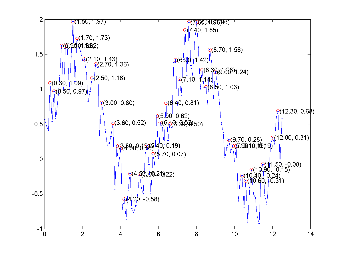
- Plot and annotate local maxima:
In this exercise, you are going to identify and annotate local maxima.
- Plot a sine wave as follows:
t=0:0.1:4*pi;
y=sin(t)+rand(1, length(t));
plot(t, y, '.-');
- Put a circle at each local maximum.
- Use the command "text" to annotate each local maximum, as follows:
- Plot a sine wave as follows:
- Plot Bezier curves:
The concept of the Bezier curve is described in the wikipedia.
- Plot 5 randomly generated data points on the x-y plane and connect them with straight lines. Be sure to label the data points as p1, p2, p3, p4, and p5.
- Draw a 4th-order Bezier curve on top of the above 5 data points.
MATLAB程式設計:入門篇
